Tutorial for anomaly detection (DNN feature matrix)
We use the FastDVDNet model to extract suitable features for anomaly detection [1]. The outcome is a predicted frame that is subtracted from the target frame to construct a feature map that is used to create the feature matrix (see Creating handcrafted feature matrix).
Previously on PiSCAT tutorials…
Please install PiSCAT Plugins UAI (link) before running this tutorial!.
We assume the user is familiar with PiSCAT. In particular, we have previously demonstrated how to use PiSCAT’s APIs for setting up the PiSCAT modules and downloading a demo iSCAT video, performing basic checks on the acquisition process and basic data visualization and how one can use DRA and FPN for backgorund correction. We have also demonstrated how to reduce the hot pixel effects. Based on the number of available CPU cores for parallel processing, this tutorial needs 12-30 GB of computer memory (RAM) to run. We also use tensor flow, which can utilize GPU for improving the performance of the DNN training/testing.
# Only to ignore warnings
import warnings
warnings.filterwarnings('ignore')
# Setting up the path to the PiSCAT modules
import os
import sys
current_path = os.path.abspath(os.path.join('..'))
dir_path = os.path.dirname(current_path)
module_path = os.path.join(dir_path)
if module_path not in sys.path:
sys.path.append(module_path)
# Downloading a measurement video for this tutorial
from piscat.InputOutput import download_tutorial_data
download_tutorial_data('Tutorial_UAI')
# Examining the status line in a loaded/downloaded video and removing the line
from piscat.InputOutput import reading_videos
from piscat.Visualization import JupyterDisplay,JupyterSubplotDisplay
from piscat.InputOutput import read_status_line
from piscat.Preproccessing import normalization
from piscat.BackgroundCorrection import DifferentialRollingAverage
import numpy as np
data_path = os.path.join(dir_path, 'Tutorials', 'Demo data', 'UAI', '9KDa')#The path to the measurement data
df_video = reading_videos.DirectoryType(data_path, type_file='bin').return_df()
paths = df_video['Directory'].tolist()
video_names = df_video['File'].tolist()
demo_video_path = os.path.join(paths[0], video_names[0])#Selecting the first entry in the list
video_ = reading_videos.video_reader(file_name=demo_video_path, type='binary', img_width=72, img_height=72,
image_type=np.dtype('<u2'), s_frame=0, e_frame=-1)#Loading the video
video = video_[1000:90000, ...]# Trimming the data and setting it to where iSCAT measurement is started.
status_ = read_status_line.StatusLine(video)#Reading the status line
video_remove_status, status_information = status_.find_status_line()#Examining the status line & removing it
#From previous tutorials: power normalization, FPNc, DRA
video_pn, _ = normalization.Normalization(video=video_remove_status).power_normalized()
batchSize = 7000
DRA_PN = DifferentialRollingAverage(video=video_pn, batchSize=batchSize, mode_FPN='mFPN')
RVideo_PN_FPN_, _ = DRA_PN.differential_rolling(FFT_flag=False, FPN_flag=True, select_correction_axis='Both')
from piscat.Preproccessing import filtering
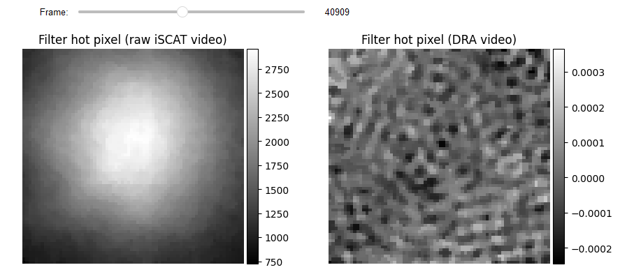
# Hot Pixels correction
video_pn_hotPixel = filtering.Filters(video_pn, inter_flag_parallel_active=False).median(3)
RVideo_PN_FPN_hotPixel = filtering.Filters(RVideo_PN_FPN_, inter_flag_parallel_active=False).median(3)
from piscat.Visualization.display_jupyter import JupyterSubplotDisplay
# For Jupyter notebooks only:
%matplotlib inline
# Display
list_titles = ['Filter hot pixel (raw iSCAT video)', 'Filter hot pixel (DRA video)']
JupyterSubplotDisplay(list_videos=[video_pn_hotPixel, RVideo_PN_FPN_hotPixel],
numRows=1, numColumns=2, list_titles=list_titles,
imgSizex=10, imgSizey=5, IntSlider_width='500px',
median_filter_flag=False, color='gray', value=40909)
   Directory  F:\PiSCAT_GitHub_public\PiSCAT\Tutorials  already exists

   The directory with the name  Demo data  already exists in the following path: F:\PiSCAT_GitHub_public\PiSCAT\Tutorials

   The data file named  UAI  already exists in the following path: F:\PiSCAT_GitHub_public\PiSCAT\Tutorials\Demo data
   ---Status line detected in column---

   start power_normalized without parallel loop---> Done

   --- start DRA + mFPN_axis: Both---
     100%|#########| 74999/74999 [00:00<?, ?it/s]

   median FPN correction without parallel loop --->
     100%|#########| 75000/75000 [00:00<?, ?it/s]

   Done

   median FPN correction without parallel loop --->
     100%|#########| 75000/75000 [00:00<?, ?it/s]
   Done

   ---start median filter without Parallel---

   ---start median filter without Parallel---
Training
Since the training process is time-consuming, especially on the CPU, and requires fine-tuning, we share pre-trained weights. Thus, you can skip to the Testing stage.
As a first step for training the fastdvdnet, the data needs to be normalized. This is done by using normalized_image_global, which renders a video with values between zero and one. FatDVDNet requires the data of the following shape: (#batches, image width, image height, #frame (always 5)),
which can be created by using the data_handling function. The output of this class can then be fed
into a tarining model.
from piscat.Preproccessing.normalization import Normalization

# Normalization
train_video = RVideo_PN_FPN_hotPixel[30000:50000:1]
video_norm = Normalization(train_video).normalized_image_global()

# Training
from piscat.Plugins.UAI.DNNModel.FastDVDNet import FastDVDNet

dnn_ = FastDVDNet(video_original=video_norm)
batch_original_array, _ = dnn_.data_handling(stride=50)

save_DNN_path = os.path.join(dir_path, 'Tutorials', 'Demo data')  # The path to the measurement data

hyperparameters = {'DNN_batch_size': 20, 'epochs': 100, 'shuffle': False, 'validation_split': 0.33}
dnn_.train(video_input_array=batch_original_array,
           DNN_param=hyperparameters,
           video_label_array=None,
           path_save=save_DNN_path, name_weights="anomaly_weights_new.h5", flag_warm_train=False)
    --- model tarin on CPU---!
    Epoch 1/100
     49/662 [=>............................] - ETA: 35:08 - loss: 0.0644
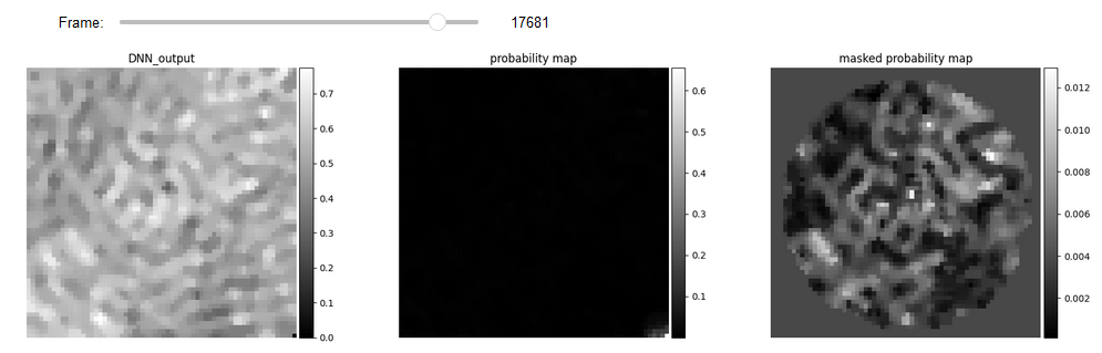
Testing
Results of DNN can be seen here. Due to artifacts that occur around edges and corners, we use the
Mask2Video class to apply a circular mask on the video.
save_DNN_path = os.path.join(dir_path, 'Tutorials', 'Demo data', 'UAI')  # The path to the measurement data

from piscat.Preproccessing.normalization import Normalization

# Normalization
test_video = RVideo_PN_FPN_hotPixel[30000:50000:1]
video_norm = Normalization(test_video).normalized_image_global()

# Training
from piscat.Plugins.UAI.DNNModel.FastDVDNet import FastDVDNet

dnn_ = FastDVDNet(video_original=video_norm)
batch_original_array, cropped_video = dnn_.data_handling(stride=1)

feature_DNN = dnn_.test(video_input_array=batch_original_array, path_save=save_DNN_path,
                        name_weights="anomaly_weights.h5")

from piscat.Preproccessing.applying_mask import Mask2Video

diff_vid = np.abs(cropped_video[2:-2, ...] - feature_DNN)
M2Vid = Mask2Video(diff_vid, mask=None, inter_flag_parallel_active=False)
circlur_mask = M2Vid.mask_generating_circle(center=(int(diff_vid.shape[1] / 2), int(diff_vid.shape[2] / 2)),
                                            redius=30)
video_mask = M2Vid.apply_mask(flag_nan=False)

# Display
list_titles = ['DNN_output', 'probability map', 'masked probability map']
JupyterSubplotDisplay(list_videos=[feature_DNN, diff_vid, video_mask],
                      numRows=1, numColumns=3, list_titles=list_titles,
                      imgSizex=20, imgSizey=20, IntSlider_width='500px',
                      median_filter_flag=True, color='gray', value=17681)
    ---Loaded model weights from disk!---
    --- model test on CPU---!
    625/625 [==============================] - 673s 1s/step
    --- Mask is not define! ---

    ---apply mask without Parallel---
      100%|#########| 19996/19996 [00:00<?, ?it/s]
      100%|#########| 19996/19996 [00:00<?, ?it/s]
from piscat.Plugins.UAI.Anomaly.hand_crafted_feature_genration import CreateFeatures

feature_maps_spatio = CreateFeatures(video=cropped_video[2:-2, ...])
dog_features = feature_maps_spatio.dog2D_creater(low_sigma=[1.7, 1.7], high_sigma=[1.8, 1.8],
                                                 internal_parallel_flag=False)

from piscat.Plugins.UAI.Anomaly.DNN_anomaly import DNNAnomaly

if_dnn = DNNAnomaly([video_mask, dog_features], contamination=0.002)
mask_video_ = if_dnn.apply_IF_spacial_temporal(step=10, stride=200)

from piscat.Preproccessing.normalization import Normalization

r_diff = int(0.5 * abs(mask_video_.shape[1] - video_norm.shape[1]))
c_diff = int(0.5 * abs(mask_video_.shape[2] - video_norm.shape[2]))

mask_video_pad = np.pad(mask_video_, ((0, 0), (r_diff, r_diff), (c_diff, c_diff)), 'constant',
                        constant_values=((0, 0), (1, 1), (1, 1)))

result_anomaly_ = mask_video_pad.copy()
result_anomaly_[mask_video_pad == -1] = 0
result_anomaly_ = Normalization(video=result_anomaly_.astype(int)).normalized_image_specific()

# Display
JupyterSubplotDisplay(list_videos=[video_norm, result_anomaly_],
                      numRows=1, numColumns=2, list_titles=['DRA', 'Anomaly'],
                      imgSizex=10, imgSizey=10, IntSlider_width='500px',
                      median_filter_flag=False, color='gray', value=17681)
    ---start DOG feature without parallel loop---
      100%|#########| 19996/19996 [00:00<?, ?it/s]

    ---start anomaly with Parallel---
      100%|#########| 19996/19996 [00:00<?, ?it/s]

    converting video bin_type to uint8---> Done
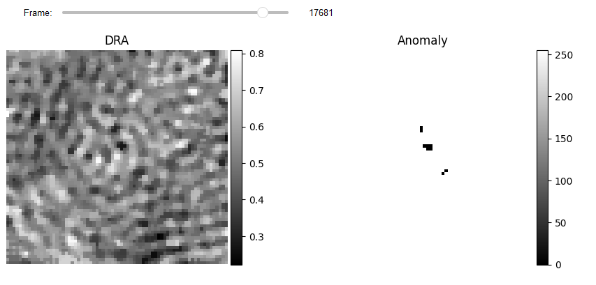
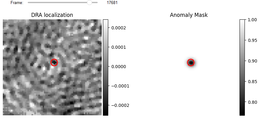
Localization
The results of anomaly detection generate a binary video with zero values for the pixels that have
been identified as anomalous. The number of connected pixels in a certain region indicates the
likelihood that this region contains an actual iPSF. The BinaryToiSCATLocalization class employs
morphological operations to eliminate low probability pixels and to determine the center of mass
for each highlighted area. Previous localization methods (e.g., DOG, 2D-Gaussian fit, and radial
symmetry) can now be utilized to fine tune localization with sub-pixel accuracy in the window
around each center of mass.
from piscat.Plugins.UAI.Anomaly.anomaly_localization import BinaryToiSCATLocalization

binery_localization = BinaryToiSCATLocalization(video_binary=result_anomaly_, sigma=1.7,
                                                video_iSCAT=test_video,
                                                area_threshold=3, internal_parallel_flag=False)

df_PSFs = binery_localization.gaussian2D_fit_iSCAT(scale=1, internal_parallel_flag=False)
df_PSFs.info()
    ---start area closing without Parallel---
      100%|#########| 19996/19996 [00:00<?, ?it/s]

    ---start gaussian filter without Parallel---

    ---start area local_minima without Parallel---
      100%|#########| 19996/19996 [00:00<?, ?it/s]

    ---Cleaning the df_PSFs that have side lobs without parallel loop---
      100%|#########| 10680/10680 [00:00<?, ?it/s]

    Number of PSFs before filters = 16813
    Number of PSFs after filters = 12071

    ---Fitting 2D gaussian without parallel loop---
      100%|#########| 12071/12071 [00:00<?, ?it/s]

    RangeIndex: 12071 entries, 0 to 12070
    Data columns (total 18 columns):
     #   Column                Non-Null Count  Dtype
    ---  ------                --------------  -----
     0   y                     12071 non-null  float64
     1   x                     12071 non-null  float64
     2   frame                 12071 non-null  float64
     3   center_intensity      9952 non-null   float64
     4   sigma                 12071 non-null  float64
     5   Sigma_ratio           12071 non-null  float64
     6   Fit_Amplitude         11612 non-null  float64
     7   Fit_X-Center          11612 non-null  float64
     8   Fit_Y-Center          11612 non-null  float64
     9   Fit_X-Sigma           11612 non-null  float64
     10  Fit_Y-Sigma           11612 non-null  float64
     11  Fit_Bias              11612 non-null  float64
     12  Fit_errors_Amplitude  11612 non-null  float64
     13  Fit_errors_X-Center   11612 non-null  float64
     14  Fit_errors_Y-Center   11612 non-null  float64
     15  Fit_errors_X-Sigma    11612 non-null  float64
     16  Fit_errors_Y-Sigma    11612 non-null  float64
     17  Fit_errors_Bias       11612 non-null  float64
    dtypes: float64(18)
    memory usage: 1.7 MB
# Localization Display
from piscat.Visualization import JupyterPSFs_subplotLocalizationDisplay
JupyterPSFs_subplotLocalizationDisplay(list_videos=[test_video, binery_localization.blure_video],
                                       list_df_PSFs=[df_PSFs, df_PSFs],
                                        numRows=1, numColumns=2,
                                        list_titles=['DRA localization', 'Anomaly Mask'],
                                        median_filter_flag=False, color='gray', imgSizex=10, imgSizey=10,
                                        IntSlider_width='400px', step=1, value=17681)
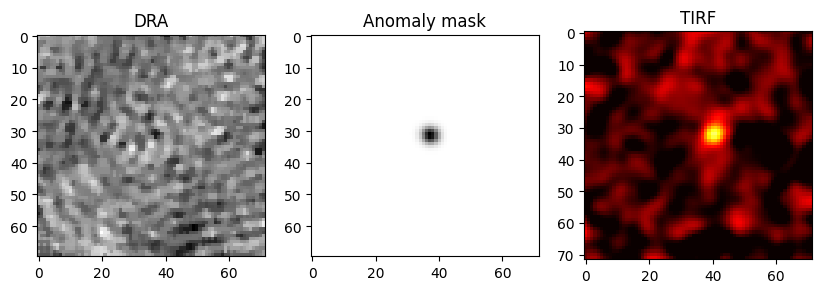
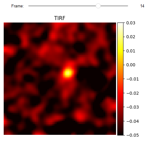
loading TIRF
To check the validity of the localization, the corresponding frames of the TIRF measurement are loaded.
data_path_Flo = os.path.join(dir_path, 'Tutorials', 'Demo data', 'UAI', 'TIRF')#The path to the measurement data
df_video_Flo = reading_videos.DirectoryType(data_path_Flo, type_file='raw').return_df()
paths_Flo = df_video_Flo['Directory'].tolist()
video_names_Flo = df_video_Flo['File'].tolist()
demo_video_path_Flo = os.path.join(paths_Flo[0], video_names_Flo[0])#Selecting the first entry in the list
video_Flo = reading_videos.video_reader(file_name=demo_video_path_Flo, type='binary', img_width=72, img_height=72,
                                    image_type=np.dtype('<f8'), s_frame=0, e_frame=-1)#Loading the video

from piscat.Preproccessing import filtering

# Hot Pixels correction
video_flo_hotPixel_ = filtering.Filters(video_Flo, inter_flag_parallel_active=False).median(3)
video_flo_hotPixel = filtering.Filters(video_flo_hotPixel_, inter_flag_parallel_active=False).gaussian(1.8)


JupyterSubplotDisplay(list_videos=[video_flo_hotPixel],
                    numRows=1, numColumns=1, list_titles=['TIRF'], imgSizex=5, imgSizey=5, IntSlider_width='500px',
                    median_filter_flag=False, color='hot', value=14, vmin=-0.05, vmax=0.03)
   ---start median filter without Parallel---

   ---start gaussian filter without Parallel---
import matplotlib.pyplot as plt
fig, (ax1, ax2, ax3) = plt.subplots(1, 3, figsize=(10,5))
ax1.imshow(test_video[17423], cmap='gray')
ax2.imshow(binery_localization.blure_video[17423], cmap='gray')
ax3.imshow(video_flo_hotPixel[14], cmap='hot', vmin=-0.05, vmax=0.03)
ax1.title.set_text('DRA')
ax2.title.set_text('Anomaly mask')
ax3.title.set_text('TIRF')
plt.show()